Image Classification with Principal Component Analysis
I recently got involved with a hack day at the University of Sussex, working on a challenge proposed by Deckchair, a company that provides high quality webcams for businesses around the world. They routinely capture some amazing images, such as lightning strikes and fireworks displays, but these are currently identified manually by eye. The challenge was to identify ‘interesting’ images automagically. Here’s a write up of my approach using Principal Component Analysis (PCA).
PCA
I chose PCA as it’s a relatively straightforward technique to understand. There are out-of-the-box implementations available in Python, useful for prototyping, and in C, in case you wish to scale.
Deckchair provided us with ~75000 low resolution RGB images from a webcam based in Venice to prototype with. To begin with I flattened the RGB images to monochrome (by taking the mean of each channel) to make the data easier to handle, and flattened the 2D array to one dimension. Using this I could extract the first 3 principal components. A monochrome image of each one is shown below.
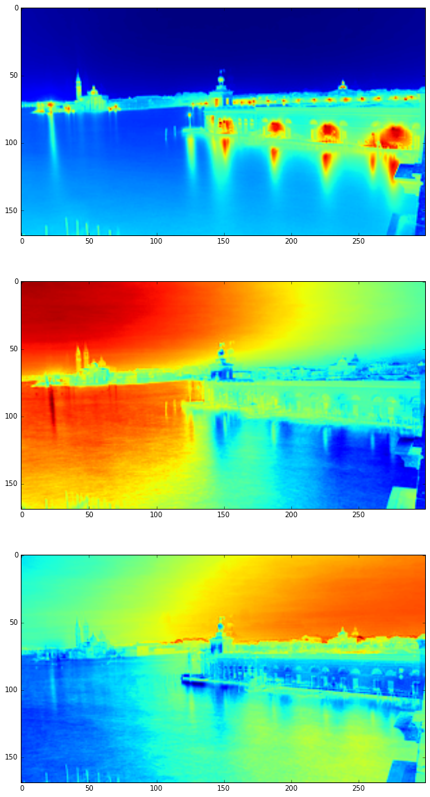
We can see some interesting patterns just from the principal components. The first principal component, which accounts for the most variability in the data, appears to highlight areas that light up after dark: windows, streetlights, reflections in the water. The second and third principal components are quite similar, showing more variation in the sky but from different directions, perhaps picking up the changes in sky colour during sunset and sunrise.
Clustering
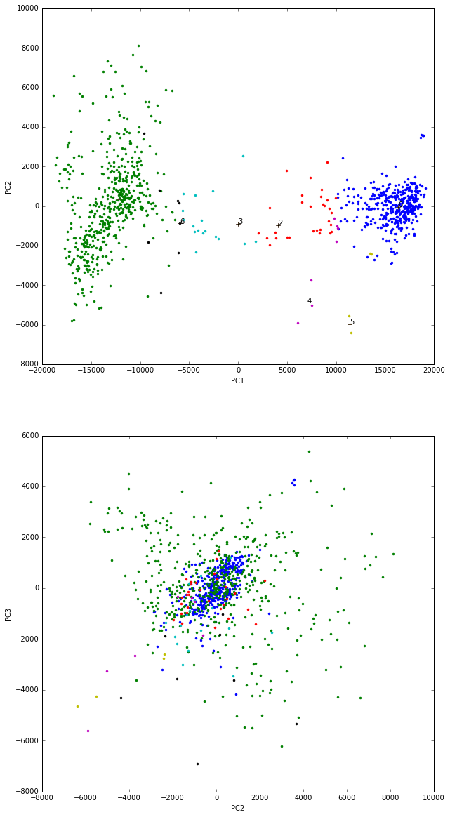
Using the meanshift algorithm we can cluster in PC space. I chose Meanshift as it’s non-parametric: you don’t need to specify up front how many clusters you want, it automatically chooses the ideal number of clusters. For an accessible introduction, see here.
Using the label data we can plot the first two PCs coloured by cluster, and with the cluster centers plotted alongside. We can also plot the 2nd and 3rd PCs against each other. Note that there is less variability in the second plot, as expected.
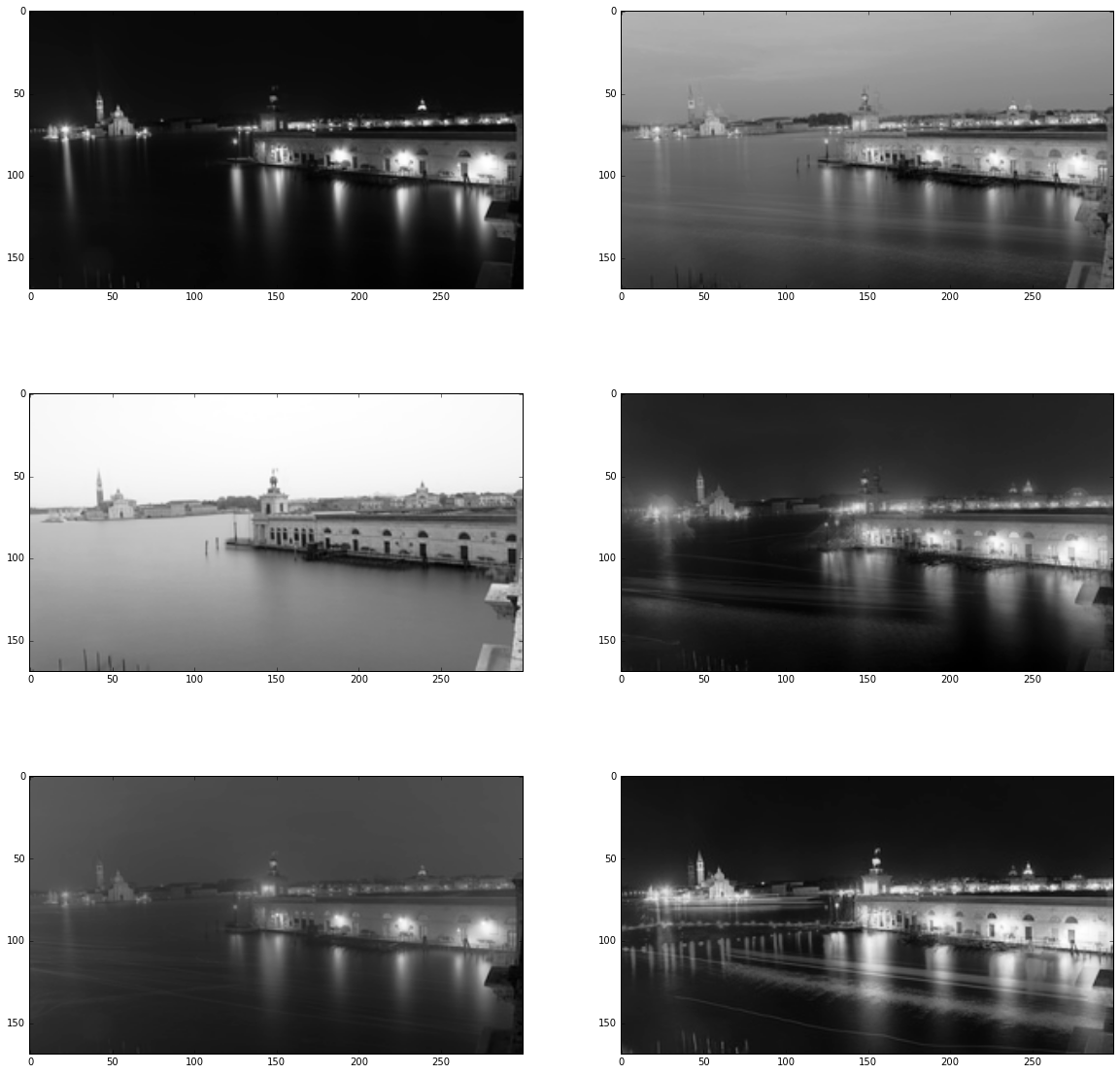
We can now go back and find the mean value of the image pixel weights in each cluster. Below is a plot of the mean image for each cluster. Note how some appear to identify night time activity, whereas others highlight water movement.
Fresh Data
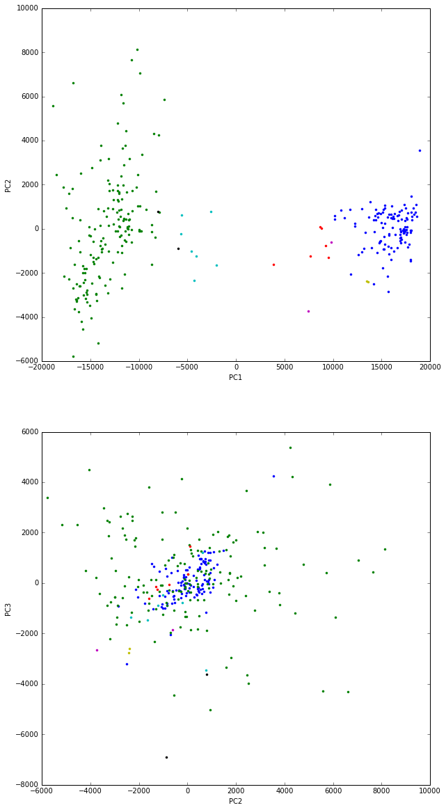
This is all well and good, but it’s only useful if we can apply our pipeline to new data. We can do this by folding a new image in to our modelled principal components to find where in this reduced dimensional space the image lies, and then classify it based on our meanshift clustering. The plot below shows the first three PCs plotted against each other, but for 1000 images not used in the component extraction or classification.
Summing Up
I’ve demonstrated how to extract the principal components from an array of images and classify in the reduced dimensional space. As an extension you could include the entire RGB array. This would take longer to extract the PCs, but the added information could aid outlier detection. I also started work on a naive outlier detector, based on distance from cluster centres.
To DIY, you can view the code here.
Subscribe via RSS