Halo mass EVS

For \(N\) haloes drawn independently from a mass distribution with PDF \(f(m)\) and CDF \(F(m)\), the PDF of the most massive is

\[\Phi(m_{\rm max}) = N \, f(m_{\rm max}) \, F(m_{\rm max})^{N-1}.\]

evstats finds \(N\), \(f\) and \(F\) by integrating a halo mass function from hmf over the comoving volume of a redshift shell, for a survey covering a fraction \(f_{\rm sky}\) of the sky. Masses are in \(M_\odot\), without factors of \(h\).

A single redshift shell

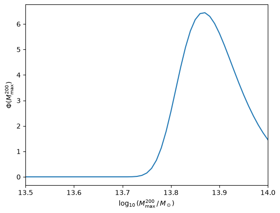
evs_bin_pdf computes the PDF for one shell, here \(4 < z < 4.4\) over the whole sky (\(f_{\rm sky} = 1\)). The hmf.MassFunction sets the mass function fit and cosmology; here the Behroozi et al. (2013) fit and Planck 2015 cosmology of Lovell et al. (2023). dz and dm set the resolution of the redshift and \(\log_{10}\) mass grids used for the integration.

import numpy as np
import h5py
import matplotlib.pyplot as plt
import astropy.units as u
from astropy.cosmology import Planck15
import hmf

from evstats import evs
from evstats.stats import compute_conf_ints

# True is the hmf default; set here to silence its warning
mf = hmf.MassFunction(hmf_model='Behroozi', cosmo_model=Planck15,
                      transfer_params={'extrapolate_with_eh': True})

pdf, log10m = evs.evs_bin_pdf(mf=mf, zmin=4.0, zmax=4.4, dz=0.01,
                              mmin=11, mmax=16, dm=0.01, fsky=1.0)

fig, ax = plt.subplots()
ax.plot(log10m, pdf)
ax.set_xlim(13.5, 14)
ax.set_xlabel(r'$\log_{10}(M^{200}_{\rm max} \,/\, M_\odot)$')
ax.set_ylabel(r'$\Phi(M^{200}_{\rm max})$');

Any survey area, across redshift

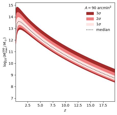
The sky fraction only enters by scaling the whole-sky \(N\), \(f\) and \(F\), which apply_fsky does. So these terms can be tabulated once, in contiguous redshift shells, and then give the PDF for any survey area almost instantly. example/data/evs_all.h5 holds them for 140 shells of width \(\Delta z = 0.2\) over \(0 < z < 28\), for the same mass function and cosmology as above. Here we take a 90 arcmin\(^2\) survey.

with h5py.File('../example/data/evs_all.h5', 'r') as hf:
    log10m = hf['log10m'][:]
    f = hf['f'][:]
    F = hf['F'][:]
    N = hf['N'][:]
    z = hf['z'][:]

fsky = float(90 * u.arcmin**2 / (4 * np.pi * u.sr))
phi_max = evs.apply_fsky(N, f, F, fsky)

compute_conf_ints gives, at each redshift, the masses at the \(-3\sigma\), \(-2\sigma\), \(-1\sigma\), median, \(+1\sigma\), \(+2\sigma\) and \(+3\sigma\) points of the CDF.

CI = compute_conf_ints(phi_max, log10m)

fig, ax = plt.subplots(figsize=(5, 5))
for i, c in enumerate(['brown', 'lightcoral', 'mistyrose']):
    ax.fill_between(z, CI[:, i], CI[:, 6 - i], color=c, label=rf'${3 - i}\sigma$')
ax.plot(z, CI[:, 3], ':k', label='median')
ax.set_xlim(0.1, 19.8)
ax.set_xlabel('$z$')
ax.set_ylabel(r'$\log_{10}(M^{200}_{\rm max} \,/\, M_\odot)$')
ax.legend(frameon=False, title=r'$A = 90\ \mathrm{arcmin}^2$');

Other mass functions and cosmologies

To use a different mass function fit or cosmology, regenerate the table with example/run_lightcone.py. It writes the same HDF5 format to example/data/, which can then be used as above:

cd example
python run_lightcone.py -o my_evs.h5 --procs 8

--model takes a preset (behroozi, the default, or yung for the Yung et al. 2024 fit) or any hmf model name, and --cosmology any astropy cosmology name; see python run_lightcone.py --help for the grid options. The table above was made with hmf 3.6; other hmf versions shift the mass function by up to ~0.2 dex at high redshift.