Stellar mass EVS

A galaxy’s stellar mass is \(M_\star = f_{\rm b} \, f_\star \, M_{\rm halo}\), where \(f_{\rm b}\) is the baryon fraction and \(f_\star\) the fraction of those baryons in stars. Following Lovell et al. (2023) we fix \(f_{\rm b} = 0.16\) and draw \(f_\star\) from a distribution. In log space the product is a sum, so the stellar mass PDF is the halo mass PDF convolved with the PDF of \(\log_{10} f_\star\), shifted by \(\log_{10} f_{\rm b}\).

First, the halo mass PDFs for a 90 arcmin\(^2\) survey, as in Halo mass EVS:

import numpy as np
import h5py
import matplotlib.pyplot as plt
import astropy.units as u

from evstats import evs
from evstats.stats import compute_conf_ints
from evstats.stellar import apply_fs_distribution, log10_fs_pdf

with h5py.File('../example/data/evs_all.h5', 'r') as hf:
    log10m = hf['log10m'][:]
    f = hf['f'][:]
    F = hf['F'][:]
    N = hf['N'][:]
    z = hf['z'][:]

fsky = float(90 * u.arcmin**2 / (4 * np.pi * u.sr))
phi_max = evs.apply_fsky(N, f, F, fsky)

Stellar fraction distributions

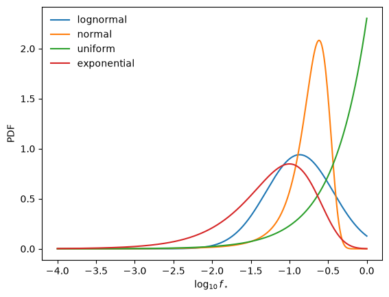
log10_fs_pdf gives the PDF of \(\log_{10} f_\star\) for each of the available distributions, truncated to \(0 < f_\star \le 1\):

v = np.linspace(-4, 0, 400)

fig, ax = plt.subplots()
for method in ['lognormal', 'normal', 'uniform', 'exponential']:
    ax.plot(v, log10_fs_pdf(v, method), label=method)
ax.set_xlabel(r'$\log_{10} f_\star$')
ax.set_ylabel('PDF')
ax.legend(frameon=False);

Stellar mass confidence intervals

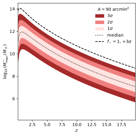
apply_fs_distribution does the convolution, here with the default lognormal \(f_\star\) distribution. Taking \(f_\star = 1\), every baryon in stars, the \(+3\sigma\) halo mass scaled by \(f_{\rm b}\) gives a conservative upper limit that is independent of the \(f_\star\) distribution (dashed line).

f_b = 0.16
mstar_pdf = np.vstack([apply_fs_distribution(p, log10m, method='lognormal', f_b=f_b)
                       for p in phi_max])
CI = compute_conf_ints(mstar_pdf, log10m)
fstar_1 = compute_conf_ints(phi_max, log10m)[:, 6] + np.log10(f_b)

fig, ax = plt.subplots(figsize=(5, 5))
for i, c in enumerate(['brown', 'lightcoral', 'mistyrose']):
    ax.fill_between(z, CI[:, i], CI[:, 6 - i], color=c, label=rf'${3 - i}\sigma$')
ax.plot(z, CI[:, 3], ':k', label='median')
ax.plot(z, fstar_1, '--k', label=r'$f_\star = 1$, $+3\sigma$')
ax.set_xlim(0.1, 19.8)
ax.set_xlabel('$z$')
ax.set_ylabel(r'$\log_{10}(M^\star_{\rm max} \,/\, M_\odot)$')
ax.legend(frameon=False, title=r'$A = 90\ \mathrm{arcmin}^2$');