Observables

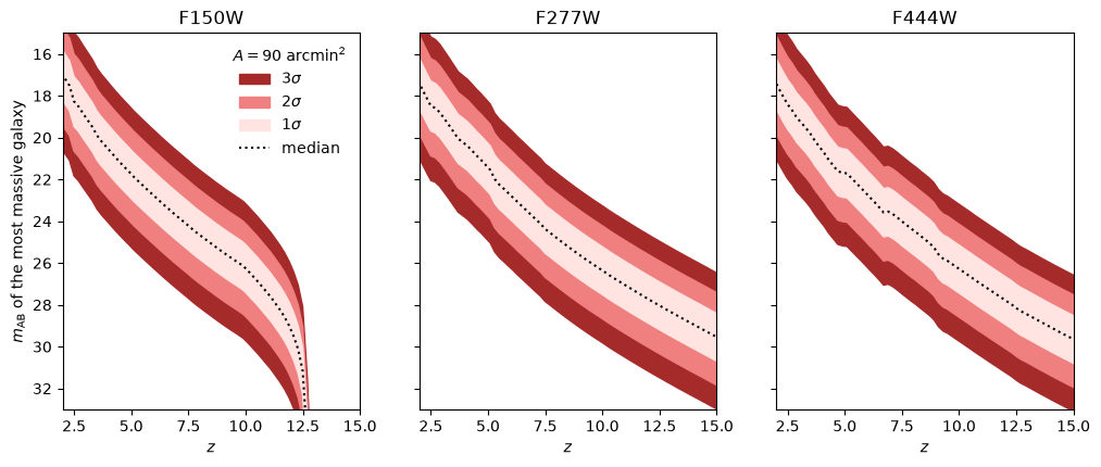
For a given stellar population model (star formation history shape, stellar population synthesis model, metallicity), a galaxy’s flux in any band is proportional to its stellar mass. A table of the flux per unit stellar mass formed, \(\mathcal{F}(z)\), therefore maps the stellar mass EVS to fluxes: the most massive galaxy has flux \(M_\star \mathcal{F}(z)\). This is monotonic in \(M_\star\), so the stellar mass confidence intervals map directly onto flux confidence intervals, which compute_conf_ints returns when given the flux at each mass as y. Mass loss from stellar evolution is neglected, so \(M_\star\) is taken as the mass formed.

example/observables/data/ includes these tables for a fiducial model, made with Synthesizer:

• an exponentially rising star formation history, \(\tau = 100\) Myr, starting at the Big Bang;

• BPASS v2.2.1 binary stellar populations with a Chabrier (2003) IMF over \(0.1\)–\(300 \, M_\odot\), plus nebular emission from Cloudy, with no escape of ionising photons;

• metallicity \(Z = 0.01\);

• Madau (1996) IGM absorption and no dust;

• JWST NIRCam F115W, F150W, F200W, F277W, F356W and F444W, and MIRI F770W;

• the Planck 2015 cosmology and the redshifts of example/data/evs_all.h5.

First, the stellar mass PDFs for a 90 arcmin\(^2\) survey, as in Stellar mass EVS:

import numpy as np
import h5py
import matplotlib.pyplot as plt
import astropy.units as u

from evstats import evs
from evstats.stats import compute_conf_ints
from evstats.stellar import apply_fs_distribution

with h5py.File('../example/data/evs_all.h5', 'r') as hf:
    log10m = hf['log10m'][:]
    f = hf['f'][:]
    F = hf['F'][:]
    N = hf['N'][:]
    z = hf['z'][:]

fsky = float(90 * u.arcmin**2 / (4 * np.pi * u.sr))
phi_max = evs.apply_fsky(N, f, F, fsky)
mstar_pdf = np.vstack([apply_fs_distribution(p, log10m, f_b=0.16) for p in phi_max])

Flux confidence intervals

For each band, the flux of a galaxy at each redshift and mass is the mass times the tabulated flux per unit mass (nJy / \(M_\odot\)), converted below to AB magnitudes. F150W drops out above \(z \approx 12\), where the Lyman break passes through it.

model = 'Exponential_tau-0.1_bpass-2.2.1-bin_chabrier03-0.1,300.0_cloudy-c23.01-sps'

fig, axes = plt.subplots(1, 3, figsize=(12, 4.5), sharey=True)
for ax, band in zip(axes, ['NIRCam.F150W', 'NIRCam.F277W', 'NIRCam.F444W']):
    fpm = np.loadtxt(f'../example/observables/data/flux_per_mass_{band}_{model}.txt')
    flux = 10**log10m * fpm[:, None]  # nJy, at each (z, log10m)
    CI = compute_conf_ints(mstar_pdf, log10m, flux)
    with np.errstate(divide='ignore'):  # zero flux beyond the Lyman break
        mag = -2.5 * np.log10(CI) + 31.4

    for i, c in enumerate(['brown', 'lightcoral', 'mistyrose']):
        ax.fill_between(z, mag[:, i], mag[:, 6 - i], color=c, label=rf'${3 - i}\sigma$')
    ax.plot(z, mag[:, 3], ':k', label='median')
    ax.set_title(band.split('.')[1])
    ax.set_xlim(2, 15)
    ax.set_xlabel('$z$')

axes[0].set_ylim(33, 15)
axes[0].set_ylabel(r'$m_{\rm AB}$ of the most massive galaxy')
axes[0].legend(frameon=False, title=r'$A = 90\ \mathrm{arcmin}^2$');

Other models

example/observables/evs_file_generator.py makes the flux tables for other star formation histories (exponential, lognormal and double power law, each over a range of parameters), stellar population synthesis models (BC03 with three IMFs, FSPS and BPASS, with and without nebular emission) and metallicities. It needs the observables extra (pip install "evstats[observables]") and the Synthesizer grids for these models; set GRID_DIR in the script to their location. Its arguments filter the star formation history, grid and metallicity, for example the fiducial grid for every star formation history:

cd example/observables
python evs_file_generator.py "" bpass-2.2.1-bin_chabrier03-0.1,300.0_cloudy 0.01

With no arguments it makes every table, which is slow. evs_sfh.py and evs_sps_imf_z.py then compare the flux predictions across these models, and evs_burstiness.py the effect of bursty star formation.